The Datasets of CeCaFLUX
|
How to prepare a model for CeCaFLUX
|
How to prepare the FTBL file for CeCaFLUX
|
Start the optimization process
|
The optimization interface of CeCaFLUX
|
The output of CeCaFLUX
|
Browser compatibility
The Datasets of CeCaFLUX
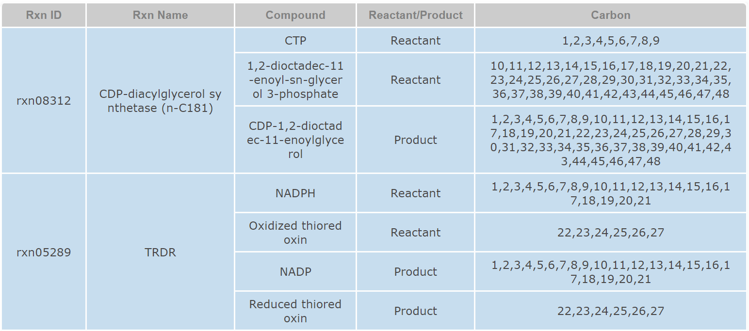
The CeCaFLUX database consists of about 551 metabolic reactions and 496 metabolites. About 100 reactions were collected from Keasling’s work while 400 reactions were collected from MetRxn Database. The central carbon metabolism reactions were from CeCaFDB. Each reaction is annotated with its popular name, stoichiometry and atom mapping information. These data can be incorporate into user’s project and facilitate their network model construction. CeCaFLUX supports standard text queries against its reactions datasets. On the reaction page, users can search through the reactions dataset using names of reaction or metabolite.
How to prepare a model for CeCaFLUX
The construction of a simulation model for CeCaFLUX relies on parsing of an input FTBL file.
Clicking the “Initialize” button on the main page or “Initialize” column on the navigation bar will create a new input page and jump to that page. An URL address was generated for this page and can be reserved by the user.
The first row of this page is a button for download of the template of the input FTBL file. The second row is for upload and parse of the user-defined FTBL file. By clicking the “Choose File” button, user can select a pre-defined FTBL from his/hers computer. By clicking the “Parsing FTBL File” button, user can upload and parse the FTBL file. The model structure, experimental measurement and 13C labeled data of the FTBL file will be converted and delivered to the server immediately. If the FTBL file can’t pass the consistency and grammar check, an error report will be displayed.

How to prepare the FTBL file for CeCaFLUX
1. Definition
The introduction about general FTBL file can be found at FIA_software_user_manual or Step-by-step tutorial for 13CFLUX software.
The CeCaFLUX FTBL file completely defines both the network and the experimental data for the 13C transient tracer experiment analysis. The file itself is a tab delimited text file, based upon the FTBL file format of the commonly used MFA estimation.
Tab-delimited files are simply tables in text format. Moving to the cell on the right (next column) is done by inserting the separator (hitting TAB), and moving to the next row is done by moving down a line (hitting ENTER). Adding comments to the file is possible by using the “//” marker. Everything in the row following this mark will be ignored.
The FTBL file is constructed out of various sections. Every section begins with the section name as the first column’s data and no other fields are filled within this row. After the section name row, its data is inserted according to the section’s format.
2. The PROJECT section
The PROJECT section is a free text section, commonly used for documentation purposes. The suggested table includes field for the name of the project, its version, date and free text comments.
3. The NETWORK section
The NETWORK section is used to define the entire stoichiometric network. The section is constructed as a table with 5 rows: FLUX_NAME, EDUCT_1, EDUCT_2, PRODUCT_1 and PRODUCT_2. Each flux is defined using 2 rows. The first indicates the flux name and its metabolic transactions. The second defines its atom transactions. Below is the definition for a flux V3 going from B + C to D.
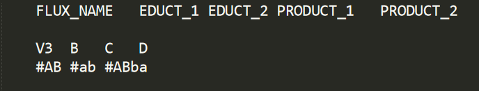
Note that since there is only one product metabolite, the column of PRODUCT_2 is left empty.
4. The FLUX section
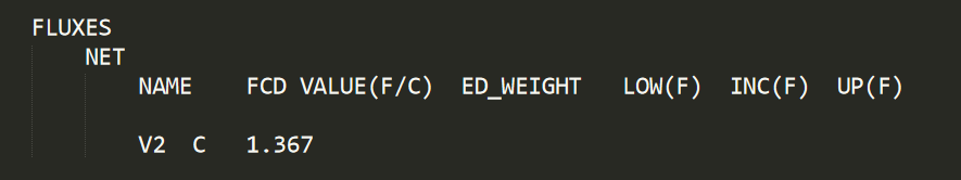
This section contains two sub sections NET and XCH. NET sub section is used to set the value for some pre-determined fluxes. A constrained flux is set to C followed by its value. Since CeCaFLUX will determine the free and dependent value automatically, the F and D symbol are meaningless here.
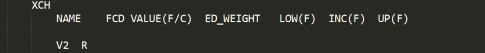
The XCH section is used to specify which reaction is reversible. The reversibility is denoted by R while irreversibility by I.
5. The EQUALITIES section
The EQUALITIES section is used to add equality constraints for the metabolic network and fluxes. In order to support the legacy of the FTBL file format, it has a subsection called NET (which is its only subsection). The EQUALITIES section contains a table with only two columns: VALUE and FORMULA. The formulas are automatically translated into their bi-directional equivalents.
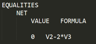
This declaration demands the value of V2 to be equal to 2 times the value of V3 (V2=3*V3).
6. The POOL_SIZE section
The POOL_SIZE section is used to supply CeCaFLUX with concentration measurements values of the metabolites. The user supplies the software the value of the measurement along with its standard deviation. For example:
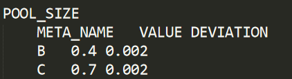
Here we supply measurement of the metabolite “B” with the value of 0.4 (units here are some factor of reactions/sec, and are usually normalized by the input flux value) and standard deviation of 0.02.
7. The LABEL_INPUT section
The LABEL_INPUT section is used to supply CeCaFLUX with known enrichments of its input fluxes. The data is supplied as follows:
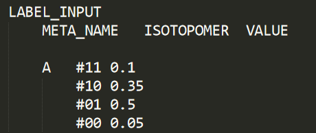
Here we provide CeCaFLUX with the isotopomer structure of the input metabolite. We specify that 50% of the input metabolite is the isotopomer 01, 5% completely unlabeled, 10% completely labeled and the rest is in 35%.
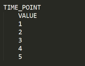
8. The TIME_POINT section
The TIME_POINT section is used to supply CeCaFLUX with the time points of the sampling for measurement.
9. The MASS SPECTROMETRY section
The MASS SPECTROMETRY section is used to supply CeCaFLUX with the data of the Mass Isotopomer measurements in a time series. Mass Isotopomer measurements specify relative strength of isotopomers, separated by the number of labeled carbon atoms in them. Time of this section has the same meaning and value as that in the TIME_POINT section. For one time point, multiple Mass Isotopomer measurements can be carried out and input for CeCaFLUX.
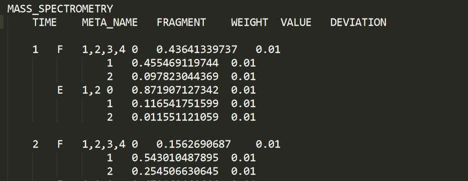
Here we can see that the m0, m1 and m2 mass isotopomers of the 1-2-3-4 (carbon atom) fragment of F was measured at time 1 and 2 with error 0.01.
Start the optimization process
The last part of input page is for specifying the parameter of optimization process. CeCaFLUX provides two methods for modeling isotope differential equations: a constant-stepsize and a Cash-Karp/Runge-Kutta method. Users can select the preferred method from a drop-down menu. For the constant-stepsize method, the user must determine the step size. For the Cash-Karp method, users must determine the relative tolerance and absolute tolerance.
After model construction, clicking the “Submit” button will start the optimization process and display to the optimization interface.

The optimization interface of CeCaFLUX
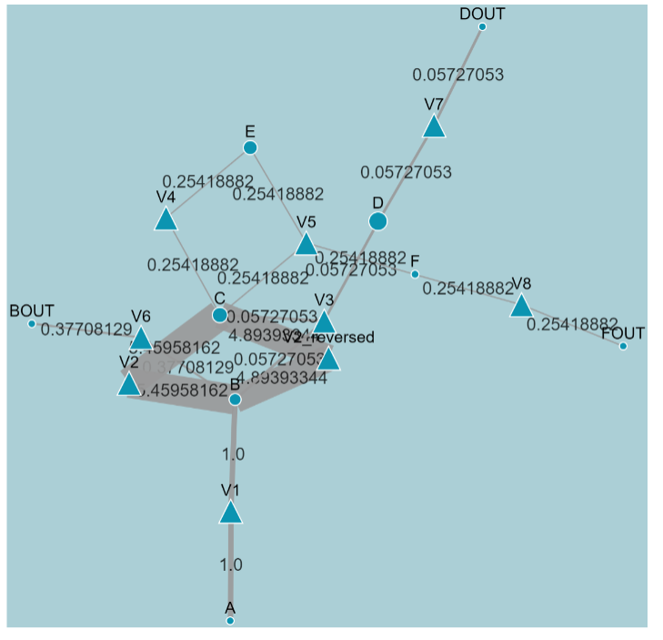
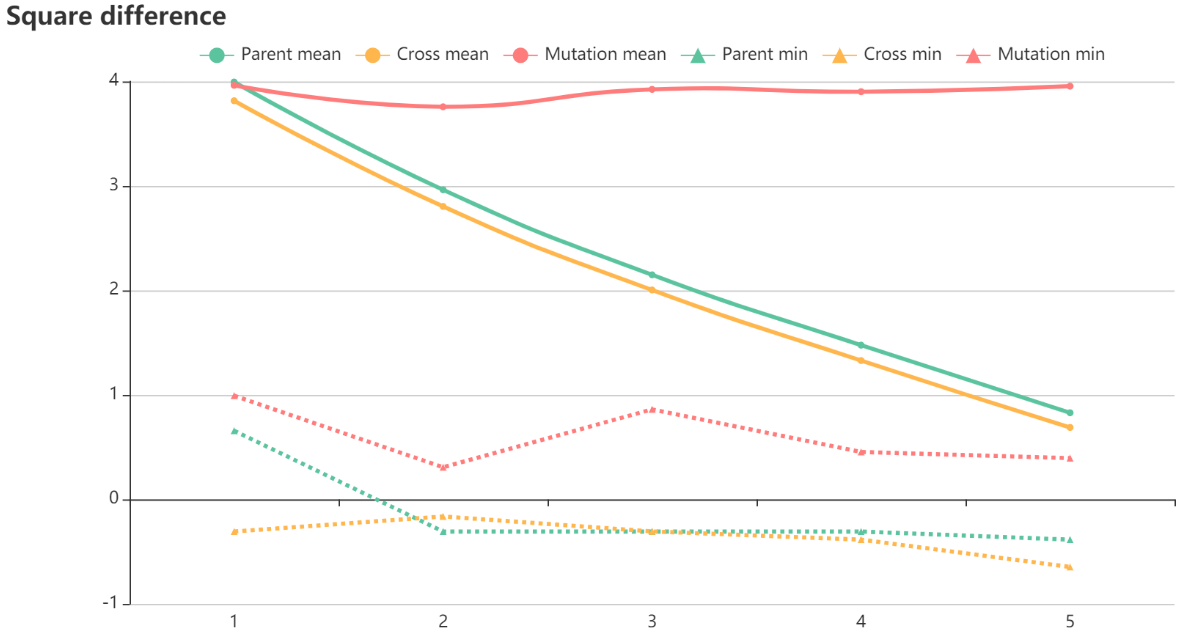
The optimization interface can be divided into 2 parts. The upper part dynamically displays the flux distribution map for each iteration. The lower part displays a line chart of the covariance-weighted sum of squared difference, where iteration number is the X-axis and the squared difference is the Y-axis. After each iteration, the adjusted flux map and its residual squares between the measured and simulated data are delivered to the graphing program using selected parameters.
The output of CeCaFLUX
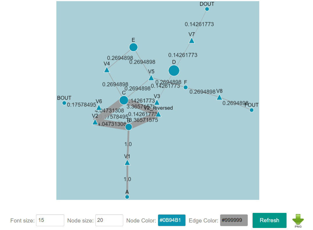
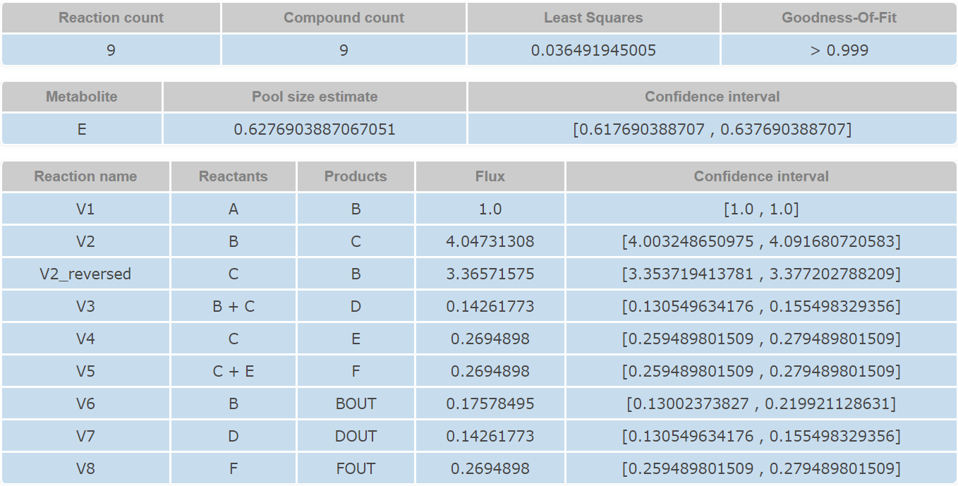
After optimization, CeCaFLUX provides an interface through which users can interactively edit and layout the nodes and edges of the flux map of the optimal values and download the graph. The output interface includes the tabular flux values, the flux graph, goodness-of-fit and the confidence intervals of the estimated parameters.
A metabolite is represented by a circle and the reaction by a triangle. An arrow denotes the direction of a reaction, and the width of the arrow is proportionate to the flux value. A force-directed layout is applied to the flux map automatically. Additionally, all the size, color, position and other element attributes can be adjusted manually. Thus, the user can manually define the appearance of the ultimate flux distribution. Clicking the “DOWNLOAD” icon downloads the current graph in .png format.
The second part provides a general description of the output result, including a summary of the network structure, including the number of reactions, number of metabolites, degree of freedom, the covariance-weighted sum of squared difference and the goodness-of-fit. The third part is a tabular representation of the ultimate flux output. The reaction names, flux value and confidence intervals are listed in this table.
Browser compatibility
The CeCaFLUX database consists of about 551 metabolic reactions and 496 metabolites. About 100 reactions were collected from Keasling’s work while 400 reactions were collected from MetRxn Database. The central carbon metabolism reactions were from CeCaFDB. Each reaction is annotated with its popular name, stoichiometry and atom mapping information. These data can be incorporate into user’s project and facilitate their network model construction. CeCaFLUX supports standard text queries against its reactions datasets. On the reaction page, users can search through the reactions dataset using names of reaction or metabolite.
How to prepare a model for CeCaFLUX
The construction of a simulation model for CeCaFLUX relies on parsing of an input FTBL file.
Clicking the “Initialize” button on the main page or “Initialize” column on the navigation bar will create a new input page and jump to that page. An URL address was generated for this page and can be reserved by the user.
The first row of this page is a button for download of the template of the input FTBL file. The second row is for upload and parse of the user-defined FTBL file. By clicking the “Choose File” button, user can select a pre-defined FTBL from his/hers computer. By clicking the “Parsing FTBL File” button, user can upload and parse the FTBL file. The model structure, experimental measurement and 13C labeled data of the FTBL file will be converted and delivered to the server immediately. If the FTBL file can’t pass the consistency and grammar check, an error report will be displayed.
How to prepare the FTBL file for CeCaFLUX
1. Definition
The introduction about general FTBL file can be found at FIA_software_user_manual or Step-by-step tutorial for 13CFLUX software.
The CeCaFLUX FTBL file completely defines both the network and the experimental data for the 13C transient tracer experiment analysis. The file itself is a tab delimited text file, based upon the FTBL file format of the commonly used MFA estimation.
Tab-delimited files are simply tables in text format. Moving to the cell on the right (next column) is done by inserting the separator (hitting TAB), and moving to the next row is done by moving down a line (hitting ENTER). Adding comments to the file is possible by using the “//” marker. Everything in the row following this mark will be ignored.
The FTBL file is constructed out of various sections. Every section begins with the section name as the first column’s data and no other fields are filled within this row. After the section name row, its data is inserted according to the section’s format.
2. The PROJECT section
The PROJECT section is a free text section, commonly used for documentation purposes. The suggested table includes field for the name of the project, its version, date and free text comments.
3. The NETWORK section
The NETWORK section is used to define the entire stoichiometric network. The section is constructed as a table with 5 rows: FLUX_NAME, EDUCT_1, EDUCT_2, PRODUCT_1 and PRODUCT_2. Each flux is defined using 2 rows. The first indicates the flux name and its metabolic transactions. The second defines its atom transactions. Below is the definition for a flux V3 going from B + C to D.
Note that since there is only one product metabolite, the column of PRODUCT_2 is left empty.
4. The FLUX section
This section contains two sub sections NET and XCH. NET sub section is used to set the value for some pre-determined fluxes. A constrained flux is set to C followed by its value. Since CeCaFLUX will determine the free and dependent value automatically, the F and D symbol are meaningless here.
The XCH section is used to specify which reaction is reversible. The reversibility is denoted by R while irreversibility by I.
5. The EQUALITIES section
The EQUALITIES section is used to add equality constraints for the metabolic network and fluxes. In order to support the legacy of the FTBL file format, it has a subsection called NET (which is its only subsection). The EQUALITIES section contains a table with only two columns: VALUE and FORMULA. The formulas are automatically translated into their bi-directional equivalents.
This declaration demands the value of V2 to be equal to 2 times the value of V3 (V2=3*V3).
6. The POOL_SIZE section
The POOL_SIZE section is used to supply CeCaFLUX with concentration measurements values of the metabolites. The user supplies the software the value of the measurement along with its standard deviation. For example:
Here we supply measurement of the metabolite “B” with the value of 0.4 (units here are some factor of reactions/sec, and are usually normalized by the input flux value) and standard deviation of 0.02.
7. The LABEL_INPUT section
The LABEL_INPUT section is used to supply CeCaFLUX with known enrichments of its input fluxes. The data is supplied as follows:
Here we provide CeCaFLUX with the isotopomer structure of the input metabolite. We specify that 50% of the input metabolite is the isotopomer 01, 5% completely unlabeled, 10% completely labeled and the rest is in 35%.
8. The TIME_POINT section
The TIME_POINT section is used to supply CeCaFLUX with the time points of the sampling for measurement.
9. The MASS SPECTROMETRY section
The MASS SPECTROMETRY section is used to supply CeCaFLUX with the data of the Mass Isotopomer measurements in a time series. Mass Isotopomer measurements specify relative strength of isotopomers, separated by the number of labeled carbon atoms in them. Time of this section has the same meaning and value as that in the TIME_POINT section. For one time point, multiple Mass Isotopomer measurements can be carried out and input for CeCaFLUX.
Here we can see that the m0, m1 and m2 mass isotopomers of the 1-2-3-4 (carbon atom) fragment of F was measured at time 1 and 2 with error 0.01.
Start the optimization process
The last part of input page is for specifying the parameter of optimization process. CeCaFLUX provides two methods for modeling isotope differential equations: a constant-stepsize and a Cash-Karp/Runge-Kutta method. Users can select the preferred method from a drop-down menu. For the constant-stepsize method, the user must determine the step size. For the Cash-Karp method, users must determine the relative tolerance and absolute tolerance.
After model construction, clicking the “Submit” button will start the optimization process and display to the optimization interface.
The optimization interface of CeCaFLUX
The optimization interface can be divided into 2 parts. The upper part dynamically displays the flux distribution map for each iteration. The lower part displays a line chart of the covariance-weighted sum of squared difference, where iteration number is the X-axis and the squared difference is the Y-axis. After each iteration, the adjusted flux map and its residual squares between the measured and simulated data are delivered to the graphing program using selected parameters.
The output of CeCaFLUX
After optimization, CeCaFLUX provides an interface through which users can interactively edit and layout the nodes and edges of the flux map of the optimal values and download the graph. The output interface includes the tabular flux values, the flux graph, goodness-of-fit and the confidence intervals of the estimated parameters.
A metabolite is represented by a circle and the reaction by a triangle. An arrow denotes the direction of a reaction, and the width of the arrow is proportionate to the flux value. A force-directed layout is applied to the flux map automatically. Additionally, all the size, color, position and other element attributes can be adjusted manually. Thus, the user can manually define the appearance of the ultimate flux distribution. Clicking the “DOWNLOAD” icon downloads the current graph in .png format.
The second part provides a general description of the output result, including a summary of the network structure, including the number of reactions, number of metabolites, degree of freedom, the covariance-weighted sum of squared difference and the goodness-of-fit. The third part is a tabular representation of the ultimate flux output. The reaction names, flux value and confidence intervals are listed in this table.
Browser compatibility
| OS | Version | Chrome | Firefox | Microsoft Edge | Safari |
| Linux | CentOS 7 |  |
|
||
| MacOS | HighSierra | |
|
|
|
| Windows | 10 | |
|
|